A Chronology of Analogue Computing
Charles Care
Introduction
Analogue computers are machines that enable a user to reason about a mathematically complex physical system through interacting with another, analogous, physical system. Distinct from digital, analogue computing was an alternative form of computer technology that had varying degrees of success. In general, analogue computers store data as a continuous physical quantity and perform computations by manipulating measures that represent numbers. On the other hand, a digital computer operates on symbolic numerals that represent numbers.1
The word ‘analogue’ was first used as a technical term during the 1940s, and referred specifically to a class of computing technology. Today, the word enjoys much wider usage, typically conveying continuity. For example, engineers will discuss analogue and digital signals, and musicians decide whether to record their work on analogue (continuous) or digital (discrete) media. As an adjective, ‘analogue’ now conveys old-fashioned and traditional, while ‘digital’ is used to signify a modern and progressive technology or medium.
However, ‘analogue’ did not always refer to the differences between discrete and continuous representation. The word analogue derives from analogy, and analogue computers were so-called because they were used to build models that created a mapping between two physical phenomena.
Analogue computing emerged during the nineteenth century and became a mainstream computing technology during the early twentieth. Since analogue was the dominant form of hardware for automatic computing between 1920 and 1940, historians of computing often consider this period to be the ‘heyday’ for analogue computing.2 In this period, the major mechanical analogue computer was Vannevar Bush’s differential analyzer, the best known of all the analogue machines developed at the Massachusetts Institute of Technology (MIT) before World War II. The differential analyser was unveiled during the early 1930s and a number of copies were made throughout the US and Europe.
Given the success of digital computers and their importance in our culture, it is tempting to assume that digital was always the better choice. However, the emergence of digital computing in the post-war period did not result in an immediate displacement of analogue computing. Around 1990, a number of scholars began to reconsider the role of analogue computing in the history of the computer. In particular their work has re-established a position for analogue within the historiography of post-1940 computing, a topic that previously had received little attention. Of this literature, James Small’s monograph The Analogue Alternative provides extensive coverage of how the differential analyser developed into an electronic-based technology, and how this technology (often known in context as the ‘general-purpose analogue computer’, or GPAC) developed during the second half of the twentieth century. Small shows that analogue computing had significant application well into the late 1970s, and illustrates how a seemingly failed technology had a strong persistence.3
Just as analogue computers did not immediately disappear, but were gradually absorbed into different genres of technologies, neither did they suddenly appear. Analogue computers belong to a rich history of calculating and modelling technologies. This article frames the development of analogue computers within a chronology of evolving technologies.4
It is common to consider the Kelvin tide predictor as the first major milestone in the development that led to the invention of the MIT differential analyser, and therefore as a beginning of a chronology on analogue computing. However, Kelvin’s machine was itself building on around sixty years of development of one of the key components of mechanical analogue computers, the mechanical integrator or planimeter. In a more popular account of analogue computer evolution, Bromley noted that because integrators provide a means for accumulating a value over the course of a calculation, they have a similar role to memory in a digital computer, and are therefore very important.5
Bromley’s account emphasises the pre-history in which planimeters, slide rules, and orrerys feature heavily. The recent scholarship referred to above has provided the opportunity to be more accurate and understand analogue computing not just a pre-history to the differential analyser. This chronology attempts a fresh analysis.
Motivation for a Parallel Chronology
A common approach to classifying the different kinds of analogue computing is to partition the technology according to whether a machine is ‘direct’ or ‘indirect’. ‘Indirect’ relates to constructing a system analogous to a mathematical (hence indirect) system such as a set of differential equations.6 Direct analogue computing represented a tradition that grew out of scientific modelling. Rather than relying on mathematical formulation, with the direct approach a relationship between two systems is set up such that a system based in one medium can be thought of an analogy of another. While the direct/indirect distinction has proved useful, it is possible that the same machine might be interpreted as both indirect and direct by different users. On closer inspection, the distinction really represents two perspectives of use.7
The intention of this article is to communicate that the chronology of analogue computing is not a uni-linear development of one central theme, but is the result of an unfolding relationship between continuous calculating devices or equation solvers and the technologies developed for modelling. To capture this plurality, the chronology is structured into three thematic time lines: the first describes the invention of the equation solvers and the second focuses on the perspective of modelling and analogy-making. The third time line takes up the story from the point when the two perspectives became unified by the common theme of ‘computing’. From here, the analogue computer developed as an alternative computing technology, and the technical terms of analogue and digital were transferred into other disciplines such as communications engineering.
Time-Line 1: Prehistory of the Origin of Continuous Computing Technology or the Development of Mechanising the Calculus
The computer as we know it today, a programmable and digital machine, emerged during the middle of the twentieth century. However, throughout history, computing tasks have been supported by a variety of technologies, and the so-called ‘computer revolution’ owes much to the legacy of the various calculating aids developed in the preceding centuries. The history of the development of various artefacts, ranging from practical astronomical tools such as the astrolabe through to more abstract calculation devices such as Napier’s bones and the slide rule, is part of a larger story. Using material culture to embody aspects of theory, these mechanisations encoded particular mathematical operations, equations, or behaviours into physical artefacts.
A mechanism to perform basic addition was first proposed in the seventeenth century; however, producing a mechanisation of higher mathematical operations such as differentiation and integration remained unsolved until the early 1800s. This thread of our chronology follows the emergence of mechanical integrators, a physical embodiment of the calculus that could be harnessed to solve systems of differential equations. As it turned out, mechanical embodiments of integration were far more straightforward to engineer for the class of technologies that came to be known as ‘analogue’; hence the major users of analogue computing were engineers and scientists interesting in solving differential equations.8
Like many other technologies in the history of computing, the integrator was adapted from another device. This device was the planimeter, a mechanically simple but conceptually complex instrument that was used to evaluate area. Our story therefore begins with the invention of the planimeter in 1818.9 The technology of the mechanical integrators inspired the development of a number of related inventions, leading to the emergence in the late nineteenth century of the ‘continuous calculating machine’.
1818–1850: The invention, reinvention and development of the planimeter
The history of science is scattered with examples of concepts being re-invented by isolated communities, and something in the technical and social climate of the early nineteenth century inspired a whole generation of area calculating instruments (or planimeters) to be invented. Before 1818, there were no instruments available to evaluate the area of land on a map or the area under a curve; by 1900, production lines were manufacturing them by the thousand.10
It is interesting to consider why there was such a high demand for the manufacture of planimeters. One reason given by contemporary sources is the sheer number of land areas that needed to be evaluated for taxation and land registry purposes. It is perhaps no coincidence that the early inventors were land surveyors and engineers. By the 1850s, one writer estimated that, in Europe alone, there were over six billion land areas requiring annual evaluation.11
Hermann, Gonnella, Oppikofer: the various inventors of the planimeter
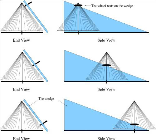
The planimeter mechanism was first invented in 1818 by a Bavarian land surveyor, Johann Martin Hermann, and subsequently went through a period of re-invention. Hermann’s planimeter consisted of a cone and wheel mechanism mounted on a track.
The actual instrument constructed by Hermann disappeared during the mid-nineteenth century, but we do have an original diagram of one elevation of the planimeter (Figures 1 and 2). In the diagram, the cone is shown side-on (the yellow triangle), and rotates in proportion with the left to right displacement of the pointer shaft. As the pen moves in and out of the drawing, the cone moves along a track (the blue rectangle). This pulls the wheel over a wedge (shown in blue on both diagrams) causing the wheel to move up and down the cone. Since the cone and wheel form a variable gear, the rate of the wheel’s rotation is dependent on both the rate of change of the wheel and the displacement of the wheel along the track. This enables the device to function as an area calculator or integrator.
The work of Hermann appears not to have been widely known until 1855 when a history of the planimeter was published by Bauenfeind. 12
Meanwhile, the idea was re-invented by the Italian mathematician Tito Gonnella (1794–1867). Gonnella was a professor at the University of Florence (Italy) and developed planimeters based around a similar cone and wheel mechanism in 1824. Later, he developed his ideas to use a wheel and disc mechanism, a copy of which was presented to the Court of the Grand Duke of Tuscany.13 Gonnella was the first to publish an account of a planimeter.14
The final ‘re-invention’ of the planimeter is attributed to the Swiss inventor Johannes Oppikofer in 1827. Oppikofer’s design was manufactured in France by Ernst around 1836 and became a well known mechanism.15 Since this planimeter also used a cone as the basic component of the variable gear, it is unclear to what extent Oppikofer’s design was an original contribution. Although it is unlikely that the instrument was copied from Hermann, there is evidence to show that it may have been inspired by Gonnella’s design.16
The development of the planimeter
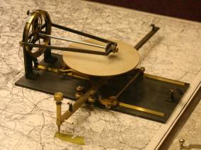
Although the idea of using a wheel and disk mechanism as the variable gear within a planimeter was attributed to the work of Gonnella, the first wheel and disk mechanism to be widely used was a planimeter designed by the Swiss engineer Kaspar Wetli.
Wetli’s planimeter was manufactured by Georg Christoph Starke in Vienna and is the archetypal wheel-and-disc planimeter. Like Gonnella’s it was exhibited at the Great Exhibition of 1851 and shown to trace areas with high accuracy. The instrument works by moving a disc underneath a stationary integrating wheel, creating the variable gear necessary for mechanical integration. The disc is on a carriage connected to the tracing point. Motion of the tracing point in one direction causes the carriage to move (changing the gear ratio between the wheel and the disc) and motion in the other direction causes the disc to spin.
In the early twentieth century, the wheel and disc integrator would become a vital component in the differential analyzer developed at MIT.
1850–1876: Maxwell, Thomson and Kelvin: the emergence of the integrator as a computing component
It was at the Great Exhibition of the works of all nations, held at Crystal Palace, London in 1851, that the natural philosopher James Clerk Maxwell first came across the planimeter which, as he later wrote, ‘greatly excited my imagination’. Enchanted by the principles behind the instrument, he began to think of further improvements.17
Maxwell’s starting point was Sang’s platometer,18 a cone and wheel mechanism designed to measure areas on maps and other engineering drawings. He found the limitations imposed by friction to be particularly frustrating and set about developing a planimeter that employed pure rolling rather than a combination of rolling and slipping. Instead of constructing a variable gear with a slipping and sliding wheel like all the other inventors before him, Maxwell’s instrument used a sphere rolling over a hemisphere. Like Sang, he published his work with the Royal Scottish Society of Arts (RSSA), who offered him a grant of ten pounds ‘to defray the expenses’ of construction.
Despite the offer of a grant, Maxwell did not pursue the development of an actual instrument. This was probably because his father warned him that the cost of such a mechanism would far exceed his budget.19 It is also evident that Maxwell had no real incentive to construct a working instrument and was more interested in the theory of the instrument. For example, when James Thomson, a Scottish engineer, published a simpler and more practical version with a perfectly acceptable accuracy, Maxwell wrote him a letter offering suggestions of how to avoid the friction he had introduced.20 Thomson’s goal had been to incorporate pure rolling in a practical mechanism and settled on a design using a sphere and disc. Maxwell’s goal was to design a theoretically elegant instrument.
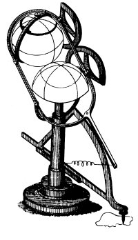
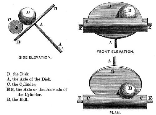
Earlier it was identified that integrators, first mechanical and then electronic would become an important enabling technology for analogue computing.21 According to the Oxford English Dictionary, the 1876 paper describing Thomson’s invention is the first occurrence of the word ‘integrator’ in English.22 With the benefit of hindsight and a little knowledge of the history of analogue computing, the key role of the mechanical integrator can appear quite obvious. However, when James Thomson first designed his integrator, there were no proto-analogue computers to employ the technology; understanding the significance of such a mechanism needed not just inventiveness but also a personal drive to mechanise calculation. Well over a decade passed before his brother, the eminent Lord Kelvin (Sir William Thomson), would provide the necessary insight, securing a place in history for the disc-ball-cylinder integrator.
During 1876, Kelvin discussed with his brother the idea of automating Fourier analysis. Kelvin had just returned from the annual meeting of the British Association for the Advancement of Science and was determined to find a solution for a problem that ‘ought to be accomplished by some simple mechanical means’. He outlined his ideas to Thomson, who in return mentioned the disc, ball and cylinder integrator. In a flash of inspiration Kelvin saw how the mechanical integrator could offer ‘a much simpler means of attaining my special object than anything I had been able to think of previously’.23
From this revelation, Kelvin moved with rapid speed. Within days, four influential papers were prepared to be given before the Royal Society of London. The first was written by Thomson and described his integrator in detail; the remainder were by Lord Kelvin and discussed their uses. These papers testify to the significance of the mechanical integrator, broadcasting to the world of science that it was possible to integrate products, solve second order differential equations, and with a particular set-up, solve differential equations of an arbitrary order. His last paper concluded with a powerful remark about the significance of the mechanisation:24
Thus we have a complete mechanical integration of the problem of finding the free motions of any number of mutually influencing particles, not restricted by any of the approximate suppositions which the analytical treatment of the lunar and planetary theories requires.25
It was not long before Kelvin’s insight was incorporated into the harmonic analyser. In use, the harmonic analyzer derived the composite harmonics of tidal data and solved equations at the Meteorological Office. As a technology, it ushered in a new genre of calculating instrument, the continuous calculating machine.
1876–1910: The age of the continuous calculating machine
Although the word ‘analogue’ was not used to refer to the devices described here (at this time ‘analogue’ referred only to analogy), the idea of a continuous calculating machine did exist. The title was used within the British scientific circle, and may have been more widely adopted, to refer to devices like the planimeter and the harmonic analyser that represented data as a physical quantity.
Working in London at what is now Imperial College, Prof. Hele Shaw had advanced the design of integrator mechanisms and understood the distinction between these devices and the numerical calculating machines available for mechanising basic arithmetical tasks. At a meeting of the Physical Society, Shaw presented a paper reviewing the various classes of mechanical integrators. While this paper is an interesting source for understanding the various technologies available for mechanising integration, it is mentioned here because of the discussion that appears afterwards, in particular the comments that Henry Prevost Babbage, the youngest son of Charles Babbage,26 directed towards Hele Shaw:
Major-General H. P. Babbage remarked that that which most interested him was the contrast between arithmetical calculating machines and these integrators. In the first there was absolute accuracy of result, and the same with all operators; and there were mechanical means for correcting, to a certain extent, slackness of the machinery. Friction too had to be avoided. In the other instruments nearly all this was reversed, and it would seem that with the multiplication of reliable calculating machines, all except the simplest planimeters would become obsolete…
[Professor Shaw] was obliged to express his disagreement with the opinion of General Babbage, that all integrators except the simplest planimeters would become obsolete and give place to arithmetical calculating machines. Continuous and discontinuous calculating machines, as they had respectively been called, had entirely different kinds of operation to perform, and there was a wide field for employment of both. All efforts to employ a mere combination of trains of wheelwork for such operations as were required in continuous integrators had hitherto entirely failed, and the Author did not see how it was possible to deal in this way with the continuously varying quantities which came in to the problem, No doubt the mechanical difficulties were great, but that they were not insuperable was probed by the daily use of the disk, globe and cylinder of Professor James Thomson in connection with tidal calculations and meteorological work, and, indeed this of itself was sufficient refutation of General Babbage’s view.27
Henry’s whole life was framed by the Babbage dream. When he was born in 1824, his father’s interest in engines was entering an intense period. Charles Babbage had successfully built a prototype difference engine in 1822 and would before long be receiving funding of £1500 to develop the full-scale model.28 Charles Babbage’s wife had died young and as a result, Henry spent most of his school years living with his grandmother before embarking on a career with the East India Company’s Bengal Army.29 He returned to England in 1874 and in retirement held a number of civic posts such as the Elective Auditor of Cheltenham, and communicating his father’s work on calculating engines. 30 During the 1880s he assembled pieces of his father’s machine and gifted them to several learned institutions including Cambridge, University College London, and Harvard University.31 He died in January 1918, aged 93.
Was Henry Babbage correct to criticise Shaw’s view of analogue technology? In many ways, Babbage should be respected for his commitment to digital, and in the long term his view ran true. However, since a reliable digital computer was not be invented until the 1940s, Shaw’s position was dominant for over 50 years. While the potential benefits of digital could be seen by visionaries, many advances in technology, coupled with a significant research budget, would be needed to realise the digital vision.
1884: Determining the engine speed of a Royal Navy warship: the Blythswood Speed Indicator, an example of embedded integrators
As well as being used in calculating devices, mechanical integrators would become embedded in real-time calculation systems, initiating the class of technology known today as control systems. An early such device was the Blythswood indicator, an instrument to measure the speed of a ship’s propeller shaft.
In a paper communicated to the Physical Society of London, engineers Sir Archibald Campbell and W. T. Goolden described a device developed for measuring the angular velocity of a propeller shaft. Their paper records how, on a visit to the dockyards of the Royal Navy in 1883, they had been drawn to the ‘very urgent need’ for an engine speed indicator.32 The issue was that to offer increased speed and manoeuvrability, ships were being built with two engines driving separate propellers. This led to the difficulty that two separate engineering systems had to be coordinated a challenge when they were located in separate engine rooms. The idea behind the Blythswood indicator was to measure the speed of the propellers automatically, and to communicate the data back to a central location from where both engine rooms could be managed.
The speed indicator is interesting because it is an early example of an integrator mechanism being embedded into an engineering system. It employed a cone and wheel in the same way as the planimeters had done previously: the cone was rotated at steady speed and the wheel shaft at engine speed, forcing the wheel to travel along the surface of the cone until the mechanical constraints imposed by the integrator were satisfied. The speed of the engine was read by measuring the displacement of this wheel (differentiating a velocity results in a displacement). The inventors then used a series of electrical contacts to sense the location of the wheel and drive a repeater instrument at a remote location.
1900–1915: Fire control in the Royal Navy: the Pollen machine
Calculations relating to ballistics problems such as the trajectories of shells constitute one of the most established uses of applied mathematics. However, during the early twentieth century advances in gunnery led to ranges measured in miles rather than yards. This meant that warships now had to engage in battle at greater distances. Over such distances, variables such as the relative speed and heading of the target ship, ship’s pitch and roll, and wind speed became important factors. Dominance in battle was no longer simply a matter of possessing the best guns and fastest ships; a warship also needed advanced computing methods.33
In terms of computation, there were two main approaches to solving the problem of calculation. The first was table-making, where the important variables (such as air speed, direction, speed of target etc.) were tabulated. A gunnery officer would be trained to look up the relevant row of data quickly, and ‘read off’ the pre-calculated settings for his gun. The alternative to using tables was to build a real-time system to calculate the correct gun settings: a machine whose mechanism reflected the actual relationships between different variables in the problem domain.34 Analogue computers were used for both approaches, differential analyzers being used extensively in the preparation of ballistic tables.
One of the earliest fire control systems was designed for the British Royal Navy by Arthur Hungerford Pollen. Pollen had invented a number of weapons systems for warships and had been introduced by Kelvin to the Thomson integrator in 1904. So when Pollen turned his mind towards the problems of fire control, it was with integrators that he pieced together his system.35
Pollen found it difficult to market his instrument to the Royal Navy, who had very conservative views towards automation. However, he did have some vindication in the performance of his system. The World War I sea battle of Jutland in May 1916 was a famous defeat for the Royal Navy, who were unable to compete against the German long range gunnery. This was partly due to a lack of gunnery computing devices: the one ship that was fitted with the Pollen system outperformed the rest of the fleet.36
1915: Technology transfer: Elmer Sperry, Hannibal Ford and fire control in the US Navy
For various reasons, fire control would find a more natural home on American warships. The principle inventor of the analogue computers used for fire control in the US was Hannibal Ford, who in 1903 had graduated from Cornell with a degree in mechanical engineering. His first employer was the J. G. White Company, where he developed mechanisms to control the speed of trains on the New York subway. In 1909 Ford began working for G. Sperry, assisting with the development of a naval gyroscope; when Elmer Sperry formed the Sperry Gyroscope Company the following year, Ford became both its first employee and chief engineer. Within Sperry, he enjoyed working closely with the US Navy developing early fire control technology; this eventually led to the establishment of his own venture, the Ford Instrument Company, in 1915.37
While working at Sperry, Ford had been given access to the designs of the Pollen system and so it is perhaps unsurprising that his mechanical integrator should be derived from the Thomson integrator. Drawing from his expertise on speed controllers, he made significant modifications to improve the torque output of the integrator, principally by adding an extra sphere and compressing the mechanism with heavy springs.38
1920–1940: The ‘heyday’ of
analogue computing?
1931 Vannevar Bush and the Differential Analyzer
Although Kelvin conceived of how mechanical integrators could be connected together to solve differential equations, a device that employed the principle was not available until Vannevar Bush invented the differential analyzer.
To solve higher orders of differential equation, it was necessary to integrate the result of a previous integration, or to allow the output of one integrator to drive the input of another. Furthermore, to solve an equation automatically, Kelvin’s machine would require a feedback loop. What Kelvin required was a torque amplifier to provide the extra turning force required, allowing a feedback loop to be set up. The torque amplifier used by Bush in the differential analyser was developed by Niemann at the Bethlehem Steel Corporation.39
Vannevar Bush (1870–1974) is well known for his contribution to twentieth century American science. He was a superb administrator and during World War II was the chief scientific advisor to President Roosevelt.
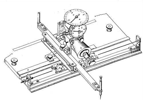
Bush’s involvement with analogue computing began during his masters degree when he developed the profile tracer, an instrument that, when pushed along, would record changes in ground level. The principle component of the profile tracer was a mechanical integrator much like Wetli’s planimeter (see above). He joined MIT in 1919, and initiated a research program that developed a variety of integrator-based calculating machines including the Product Integraph and the Differential Analyzer.40
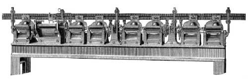
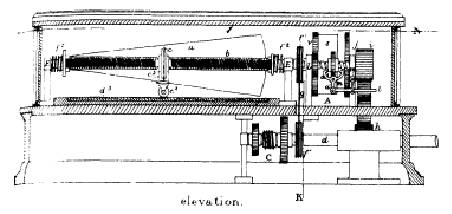
The differential analyzer was completed between 1930 and 1931. It was the size of a large table with long shafts running down its centre. Along these shafts were eight mechanical integrators and a number of input and output tables. By using the different shafts to connect together the inputs and outputs of the different functional components, it was possible to construct a system governed by a differential equation.41
During the late 1930s, MIT was supported by the Rockefeller foundation to construct a larger and more accurate machine. The Rockefeller Analyzer, as it was known, would still employ mechanical integrators, but used servo mechanisms to speed up the programming of the machine.42
Time-line 2: From experiment to computation: the development of electrical modelling technologies
There are two main aspects to analogue computing: the use of continuous representation and the employment of an analogy. Looking at the history of the mechanical integrator gave us a history of the continuous calculating machine; now we will turn to the tradition of analogue computing that emphasises the construction of analogies.
The idea of an analogue system is more closely related to the tradition of modelling in the natural sciences than to the history of calculating machines. For generations scientists have constructed models to illustrate theories and to reduce complex situations into an experimental medium.43 Since the mid-nineteenth century, the technology available for creating models (or analogies) has become part of the history of computing, developing from ad-hoc laboratory set-ups and evolving into sophisticated, general purpose tools.
1845–1930: Nineteenth century physics meets nineteenth engineering: the development of analogy methods
During the nineteenth century, model construction was presented with a new medium, that of electricity. Using electrical components for modelling offered improved flexibility and extended the scope of what could be represented in a machine. In many ways, the history of the development of modern computing can be understood as the endeavour of trying to manage an electrical (and later electronic) modelling medium.
For the history of analogue computing, modelling techniques using electrical methods were either circuit models, of which the Network Analyser became an archetype, or, alternatively, set-ups exploiting the physical shapes and properties of a conducting medium such as conducting paper or electrolytic tanks. Together, these techniques became known as electrical analogy methods, the models being referred to as ‘electrical analogies’ and later as ‘electrical analogues’.
1845 Kirchhoff and conducting paper
Identifying that lines of electrical flux could represent flow dates back to some early work by the German physicist, Gustav Robert Kirchhoff. Kirchhoff used conducting paper to explore the distribution of potential in an electrical field. The so-called field plot turned an invisible phenomena into a visual diagram and allowed scientists to begin exploring the analogy between fluid flow and electrical fields.44
1876 William Grylls Adams and the electrolytic tank
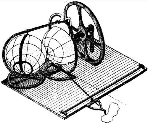
In the same volume of the Transactions of the Royal Society where Kelvin demonstrated how an integrator could solve differential equations, a different form of modelling technology was communicated to members of the Royal Society.45 This was an electrolytic tank developed by the British scientist, William Grylls Adams, and would later become an important example of analogue computing.
Adams was the younger brother of John Crouch Adams, the astronomer who discovered the planet Neptune. He spent most of his academic career at King’s College, London, firstly as a lecturer and then, from 1865 to 1905, as a professor of natural philosophy and astronomy (the chair previously held by James Clerk Maxwell.) At King’s, Adams established the Physical Laboratory (1868) and was committed to both teaching and research in experimental physics.46
Adams’ tank further contributed to the approach of visualising electrical field lines. It consisted of a wooden tank containing water, two fixed metal electrodes, and two mobile electrodes. Connecting a power source to the fixed electrodes established an electrical field, which could then be explored with the mobile electrodes. (See Figure 10: the fixed electrodes are marked A and B, the mobile electrodes are connected to the T-shaped handles.)
1880–1920 Modelling Power Networks
In the 1880s Thomas Edison, the inventor of the light bulb, employed a research assistant to build scale models of power networks. Over a number of years, these models evolved from special purpose laboratory experiments towards more general purpose set-ups. Following a general pattern from the specific to the generic, experiments became modelling set-ups, which in turn developed into special purpose electrical analogues. Electrical analogues were replaced by programmable analogue computers before a final transition to programmable digital computers was made between 1960 and 1980.
With reference to these electrical calculations, Aristotle Tympas noted that the technology has repeatedly shifted between analogue and digital throughout history. Following the debate established by James Small’s The Analogue Alternative, Tympas observes that: ‘[T]he network analyzer, considered by contemporary scholars to be an exemplar of an analog computer, came as a savior of the calculating machine…, now considered an exemplar of a digital computer’.47
Tympas goes on to argue that the analogue/digital ‘demarcation’ was projected on to the pre-1940 period. Within the context of a separation between continuity and modelling as put forward in this article, this makes sense; however, we can take the argument further. There was a analogue/digital debate during the early 1900s over whether electrical problems should be solved with modelling techniques as opposed to numerical calculation.
1920–1940: Pre-digital analogue modelling
1924 The origin of the MIT Network Analyzer
Just as Edison had constructed scale models during the 1880s, researchers at MIT began to build special purpose models to assist with the design of new power distribution networks. Developing an individual model for each network was not very flexible; what researchers realised they needed was a more generic tool. The network analyzer occupied a room and through its patch panels, allowed a user to set up a specific network quickly. Initially the analyzer was used just to reason about electrical supply networks in miniature; however, the research team soon developed techniques for wider modelling applications, representing more exotic referents such as hydraulic systems within the framework of resistor-capacitor networks.
Techniques using resistance networks were particularly useful in geographical calculations because the layout of the problem could physically map to the geography of the real-world problem. Bush identified the network analyzer as an instrument in which whole equations mapped to a particular set-ups. By contrast, the differential analyzer established analogies between the machine and individual components of a differential equation.48
The co-evolution of network analysers and machines based on integrators came together in the research at MIT where both the Network and Differential Analyzers were developed. They represented different activities, two perspectives of use, thus sub-dividing the analogue computing class. Small saw them as competitive technologies that ‘maintained distinct lineages, but nevertheless shared a similar conclusion; their displacement by electronic digital computers’.49
George Philbrick and the Polyphemus: development of electronic modelling
Around 1940, the electronic analogue computer would be born. This technology was essentially a transition of the concepts of the differential analyzer, but fuelled by advances in control electronics and feedback systems. Many pioneers of electronic analogue computers were people who had previously undertaken research in control systems analysis or similar fields. One example is George Philbrick (1913-1974), who had worked for the Foxboro Corporation during the pre-war years before joining the fire control division of the US government’s National Defense Research Council (NDRC).
Philbrick began working for the Foxboro Company in 1936 after graduating from Harvard and worked for the control engineer Clesson E. Mason.50 While working on a complete mathematical analysis of process controller, Philbrick created the Polyphemus simulator, an early electronic computer.
In his writing and research, Philbrick contributed to technology of analogue computing and linear electronics. A recent textbook on the design of analogue electronic systems claimed it would be ‘difficult to imagine a real guide to analog design without George Philbrick’, a sentiment that is echoed across the field of electronic analogue design.51
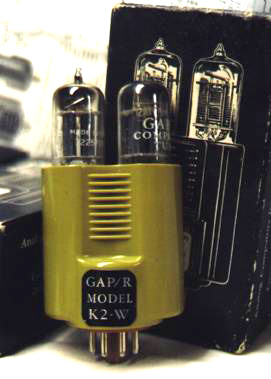
Once his wartime research was completed, Philbrick had intended to enrol at MIT as a graduate student and develop a high-speed analogue computer. However, this project was indefinitely put on hold when he was approached to design a special purpose simulator for the Wright Aeronautical Corporation. He successfully constructed the simulator in his spare bedroom and set up his own company: George A. Philbrick Researches, Inc. (often abbreviated to GAP/R), the first company to manufacture and market a commercial operational amplifier (op-amp).52
1932 Le Laboratoire de Analogies Electrique: electrolytic tanks in France
During the 1930s the French mathematician Joseph Pérès (1890–1962) had begun to use electrolytic tanks to model physical systems.53 In 1921 Pérès was appointed Professor of Rational and Applied Mechanics at Marseilles where he was inspired by the analogue modelling of his colleague J. Valensi.
Valensi’s involvement in analogue computing dated back to 1924, when he had solved a fluid dynamic problem by employing an analogy between streamlines of fluid flow and potentials in an electrical field. In 1930, Valensi and Pérès founded an Institute of Fluid Mechanics at Marseilles and, between 1930 and 1932, collaborated to research the application of electrolytic tanks for solving these problems. Around 1932 Pérès accepted a Chair at the Université Paris-Sorbonne where, with his researcher Lucian Malavard, he established a Department of Electrical Analogy (Le Laboratoire des Analogies Electriques) within the Paris Faculte des Sciences.54
In Paris, Pérès and Malavard began to develop various refinements in electrolytic tank methods. In particular they developed applications using tanks of various depths, a technique that had been employed within British aeronautical research.55 The outcome of the work was the Wing Calculator, a tank that could solve the equations governing a lifting wing. The calculator was used by a number of aircraft manufacturers until 1940, when the outbreak of war in Europe prompted the lab to be dispersed and the remaining research destroyed.56
1942 William A. Bruce and the modelling of oil reservoirs
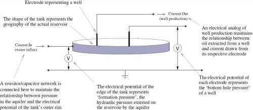
According to a history of oil reservoir simulation by Donald Peaceman, analogue techniques were used to simulate oil fields during the 1920s and 1930s. However, within the reservoir engineering literature, the first well-known application of analogue computing to such problems is attributed to William A. Bruce, a researcher of Carter Oil. He invented his ‘analyzer for subterranean fluid reservoirs’ in 1942, demonstrating that the dynamics of an underground oil reservoir could be represented by electrical circuits.57
In Bruce’s analyzer, the reservoir was modelled with an electrolytic tank using electrodes to represent the flow of fluid in the system. The edge of the tank (see Figure 12) formed one side of the circuit, representing water influx as a current flowing into the tank; a number of smaller electrodes represented the oil wells by drawing a current proportional to actual oil production.
Initially, Bruce made no reference to analogue, analogy, or computing: throughout his 1945 patent application, the circuit was described as an ‘electrical counterpart of a reservoir’. Later, reservoir analysers would employ the conceptual label of ‘electrical analogies’ and thus become aligned to the analogue computing field.58
Time-line 3: The entwining of continuity and modelling and the development of an analogue alternative
It was only after the emergence of the digital computer that it became necessary to have an umbrella term for analogue computers. According to the Oxford English Dictionary, the earliest use of the word ‘analogue’ to describe a class of computers is attributed to the British physicist Douglas Rayner Hartree. In a 1946 article, he wrote of the differences between the two classes of computer and wrote that ‘the American usage is analogue and digital machines’.59 It can be assumed that Hartree was introduced to the analog/digital classification during his visits to the Moore School of Electrical Engineering at the University of Pennsylvania and possibly from Mauchly who was using the term in communication with Atanasoff in 1941. In 1941, Mauchly made the following notes (note the use of ‘impulse’ where we would now use ‘digital’):
Computing machines may be conveniently classified as either ‘analog’ or ‘impulse’ types. The analog devices utilize some sort of analogue or analogy, such as Ohm’s Law or the polar planimeter mechanism, to effect a solution of a given equation… Impulse devices comprise all those which ‘count’ or operate upon discrete units corresponding to the integers of some number system…60
Mauchly was a member of the team at the Moore School where the ENIAC, the first programmable electronic digital computer was constructed.61 Although fundamentally a digital machine, ENIAC was in many ways an extension of the analogue culture that had existed previously. The choice of acronym (standing for Electronic Numerical Integrator and Computer) emphasises the link. We have already seen that a major application of the analogue computers was to mechanising the calculus; the ENIAC was intended to solve problems that had previously been undertaken by differential analyzer. An insightful quote from the ENIAC patent (submitted in 1947) shows that making an analogue computation was understood as akin to conducting a laboratory experiment.62 The digital ENIAC offered a ‘cleaner’, more mathematical alternative:
Those problems which cannot be solved analytically have been handled by computational methods or through the use of specific analogy machines… An exemplification of the latter techniques is found in the use of wind tunnels. At present, the supersonic wind tunnel at the Ballistic Research Laboratory, at Aberdeen, Maryland, is used about 30% of the time as an analogy machine to solve two-dimensional steady state aerodynamical problems… It may be noted that much of the present experimental work consists essentially of the solution of mathematical problems by analogy methods. If one had a computing machine of sufficient flexibility the necessity for these experiments would be obviated. Our invention makes available such a machine.
In discussing the speed of computing machines it is desirable to distinguish between so-called continuous variable and digital machines. Although existing continuous variable machines such as the differential analyzer and the AC network analyzer are exceedingly rapid, the class of problems which they can solve is limited.63
As can be seen from the quote, the 1940s was the period when the concept of the ‘analogue computer’ was introduced to encompass both of the traditions explored in our first two time-lines. Here John Mauchly and Presper Eckert, the authors of the patent, separate the technical concept of continuous variables—a defining characteristic of continuous calculating machines—and the conceptual idea of analogy, characteristic of modelling technologies.
1950–1970 The origin (and demise) of the commercial analogue computer
One of the major technical benefits of World War II was the improvements to electronic components. During the years after 1945, analogue computers were constructed using electronic components, the mechanical integrators being replaced with capacitor charging circuits. A number of companies began to manufacture analogue computers and the computers became important tools in engineering and scientific establishments.
Electronic analogues were typically used for three major applications: solving differential equations, modelling complex systems, and simulating control systems. The demise of the analogue computer was a gradual process. Apart from reductions in size and improvements in speed, the machines on sale up until 1970 were all essentially electronic differential analysers.64
Unusual analogue devicesThe following inventions, the Phillips machine and the Jerie computer, are analogue computers by association. They are quite different from other mainstream analogue computers in that they are not electronic and have a more visual quality. They are interesting, however, because they are both referred to in contemporary context as analogue computers.
For example, in a 1957 paper Jerie referred to his machine as an analogue computer. As historians, we need to respect the context of his association. If actors choose to label an artefact as an analogue computer, we can derive insight into how technical cultures perceived and understood analogue computing.
1949 Modelling an economy: The Philips MachineIn general the post war period saw analogue computing shift into the electronic realm, however the Phillips machine provides some food for thought as to how a hydraulic analogue computer might work.
In the Phillips machine, the flow of money around an economy maps to the flow of liquid around the machine. At various points during the flow, proportions of liquid could be routed off into storage vessels representing, say, national savings. Government borrowing is represented by removing money from a storage vessel.
Like many of the analogue computers described so far in this account, the machine developed by the economist A W Phillips provided an embodiment of a system of differential equations. The difference between his machine and others is that he represented variable quantities as levels of fluid.65 Although it is frequently cited as an analogue computer, recent scholarship has questioned whether this is really a computer in a general sense.66 Really what Phillips was trying to produce was a illustrative model of Keynesian economics. It perhaps does not matter too much whether such a device is a computer or not and in this aim the machine was successful.
1957 Machine supported map making: the Jerie analogue computer
Photogrammetry, the application of photography as an aid to mapping and surveying, was first pioneered during the late nineteenth century. The essential principle is that a number of photographs, taken from different angles, can be used to create a map if they share a common set of identifiable ‘control points’. During the mid 20th century, new methods were suggested but required the solution of a large system of simultaneous equations. The analogue computer proposed by Professor H. G. Jerie of the International Training Centre for Aerial Survey (ITC) in Delft, the Netherlands, was a special purpose, mechanical device for solving these problems. The computer was patented by the ICT and was marketed and manufactured with reasonable success. 67
In order to use a set of photographs for mapping, it is necessary to calculate the respective positioning of each photograph and to resolve the images by identifying known control points. This is known as aerial triangulation and at the time when Jerie invented his computational aid, a large number of control points were required in order to ‘obtain the generally desired accuracy’. By splitting up the area into blocks rather than strips as was then the custom, the problem required fewer control points to be identified; at the same time this led to a large system of simultaneous equations requiring solution. This meant that solution by numerical methods was very difficult and Jerie turned to the application of analogue computing techniques to the problem. His invention, which he referred to as an analogue computer, used a mechanical design in which the unknowns of the equations were represented by elastic connections between plates.68
The machine essentially constructed an analogue to the problem. In a typical problem many photographs will overlap, and it is necessary to resolve the different views of each image. In the Jerie computer, the various images were transferred onto overlapping plates and the control points of each plate anchored together. Other than at these anchor points, the plates were free to move within the constraints of their elastic connections, eventually stabilising on a solution that best satisfied the positional constraints between the plates.
Conclusions
This article has put forward a chronology of the development of analogue computing. Due to the number of different technologies and contexts, the coverage of individual machines and inventors has been kept deliberately short. Readers interested in the history of analogue computing in general should turn to the monographs by James Small and David Mindell, who cover many of the machines described. For those interested in specific machines, the footnotes provide an entry point into the literature.69
One of the purposes of preparing this chronology was to demonstrate the wide variety of technologies that are relevant to the history of analogue computing and to highlight that defining ‘analogue computing’ is a challenging problem. This leads to an anachronic/diachronic tension, since much of the historiography on analogue computing focuses on periods when the dichotomy analogue/digital did not exist.70
By its very nature, the development of the analogue computer does not map to a coherent linear chronology, and it is not until 1940 that various concepts are absorbed into the conceptual entity of ‘analogue computing’. This article highlights some important factors in the enclosure of analogue computing, in particular the origin of the term and the drawing together of the two technical traditions: continuous calculators and modelling tools. As we have seen, these two major themes can give coherence to what is otherwise a muddle of association. Previous work on this history has not yet taken this properly into account and tends to highlight only one of these perspectives.71
Notes
1 For the distinction between numeral, number and measure: see Donald M. MacKay and Michael E. Fisher, Analogue Computing at Ultra-High Speed, Chapman and Hall, London, 1962.
2 See Martin Campbell-Kelly and William Aspray, Computer: A History of the Information Machine, 2nd ed. Westview Press, 2004, p. 52.
3 James S. Small, The Analogue Alternative: The Electric Analogue Computer in Britain and the USA, 1930–1975, Routledge, 2001. Other significant contributions to re-establishing the history of post-war analogue computing include: William Aspray, ‘Edwin l. Harder and the Anacom: analog computing at Westinghouse,’ IEEE Annals of the History of Computing, 1993, 15(2):35 – 52; Aristotle Tympas, ‘From digital to analog and back: The ideology of intelligent machines in the history of the electrical analyzer, 1870s–1960s’, IEEE Annals of the History of Computing, 1996, 18(4):42–48 and David A. Mindell, Between Human and Machine: Feedback, Control, and Computing Before Cybernetics, The John Hopkins University Press, Baltimore, 2002.
4 Regarding the origin of a definition for analogue computing, this article shows that our current understanding of ‘analogue’ is the result of many different associations. In particular, there are a number of nineteenth century technologies understood to form its technical heritage; these are either considered as analogue computers in their own right, or understood to be early mechanisms that became assembled as components into later analogue computers.
5 Allan G. Bromley, ‘Analog computing devices’, in William Aspray, ed., Computing before Computers, Iowa State University Press, 1990, pp. 159–199 .
6 See Bromley, ‘Analog computing devices’, 1990, op. cit. and Small, The Analogue Alternative, 2001, op. cit., pp. 30–31.
7 The MIT Network Analyzer is a good example; this machine began as a generic tool for modelling power networks and was later interpreted as a calculating machine.
8 This is reflected in the name Vannevar Bush chose for what has become the most famous analogue computer: the Differential Analyzer.
9 Croarken identified that within the context of computer history, the planimeter was ‘the most significant mathematical instrument of the 19th century’. See Mary Croarken, Early Scientific Computing in Britain, Clarendon, Oxford, 1990, p.9.
10 The most popular planimeter to be manufactured would be the Amsler Polar Planimeter invented in 1854; it sold over 12,000 copies before the early 1890s. See O. Henrici, ‘Report on planimeters’, in Report of the Sixty-fourth Meeting of the British Association for the Advancement of Science, 1894, pp. 496–523.
11 Henrici, ‘Report on planimeters’, op. cit. An interesting connection is that the invention of the planimeter roughly coincides with major reform in German land law. The Gemeinheitsteilungsordnung (decree for the division of communities) of 1921 presumably increased the demand for a calculating aid. See Max Weber, General Economic History (trans. Frank H. Knight), Collier-Macmillan, 1966, pp. 28–29. Another major use was the integration of steam engine integrator diagrams.
12 See Henrici, ‘Report on planimeters’, op. cit.
13 The instrument belonging to the Grand Duke was exhibited at the Great Exhibition, Crystal Palace, London, in 1851.
14 Anon., ‘Planimeters’, Exhibition of the Works of Industry of all Nations, 1851 : Reports by the juries on the subjects in the thirty classes into which the exhibition was divided, Clowes, London, 1852; Henrici, ‘Report on planimeters’, op. cit.
15 Allan G. Bromley. ‘Analog computing devices’, 1990; Joachim Fischer. ‘Instrumente zur Mechanischen Integration: Ein Zwischenbericht, ’ in 25 Jahre Lehrstuhl für Geschichte der exakten Wissenschaften und der Technik an der Technischen Universität Berlin 1969–1994, 1995; Henri de Morin, Les Appareils D’Intégration, L’Ecole Polytechnique, Paris, 1913. Available online from Cornell Manuscript Collection http://historical.library.cornell.edu
16 There is no definite evidence that Oppikofer copied Gonnella, although Gonnella had sent his designs to a Swiss instrument maker shortly before Oppikofer’s invention had appeared. In 1894 Henrici wrote that ‘[h]ow much he had heard of Gonnella’s invention or of Hermann’s cannot now be decided’ (Henrici, ‘Report on planimeters’, op. cit.).
17 James Clerk Maxwell, ‘Draft of a paper on the Platometer’ (1855), in P.M. Harman, ed., The Scientific Letters and Papers of James Clerk Maxwell, volume I (1844–1862), Cambridge University Press, 1990, pp. 275–279.
18 The platometer was an independent invention designed by John Sang, a fellow Scotsman, during the late 1840s. A number of other planimeters were exhibited at Crystal Palace including mechanisms by Gonnella and Wetli. It is claimed that, apart from Gonella’s instrument, Sang was unaware of other planimeters at the exhibition, so it is difficult to judge which instruments Maxwell discovered there. By 1855 Maxwell was aware of Gonnella’s work in Italy and made reference to it in his paper. See Anon., ‘Report on the platometer’, Transactions of the Royal Scottish Society of Arts, (4):126–129, 1852; and James Clerk Maxwell, ‘Description of a New Form of Platometer, an Instrument for Measuring the Areas of Plane Figures’ (1855), in W.D. Niven, ed., The Scientific Papers of James Clerk Maxwell, Cambridge University Press, 1890, pp. 230– 237.
19 James Clerk Maxwell, ‘From a Letter to John Clerk Maxwell (1855)’, in P.M. Harman, ed., The Scientific Letters and Papers of James Clerk Maxwell, volume I (1844–1862), Cambridge University Press, 1990, p 325; Lewis Campbell and William Garnett, The Life of James Clerk Maxwell, Macmillan and Co., 1882, pp 114-5.
20 James Thomson, ‘An integrating machine having a new kinematic principle’, Transactions of the Royal Society of London, 24, 1876, pp. 262–265; James Clerk Maxwell, ‘Letter to James Thomson (with reply)’, in P.M. Harman, ed., The Scientific Letters and Papers of James Clerk Maxwell, volume III (1874-1879), Cambridge University Press, 2002, pp. 829–230.
21 For example, Small’s recent history of analogue computing is really a history of analogue computers employing some form of integrator. Such a reduction in scope is not noticed by its general readership and the book is considered a general history of analogue computing. This is because the class of instruments that relate to the differential analyzer—the class that Vannevar Bush referred to as ‘equation solvers’—became the single most important type of analogue computer.
22 This marks the end of a story about the planimeter, an instrument, and the beginning of the mechanical integrator, a component. The OED defines integrator as ‘one who or that which integrates’; the earliest quote that they record for either is James Thomson’s usage. ‘Integrator’ Oxford English Dictionary. 2nd ed. Oxford University Press, 1989; OED Online. http://dictionary.oed.com/cgi/entry/50118577, Accessed 1st November 2006.
23 William Thomson (Lord Kelvin), ‘On an instrument for calculating the integral of the product of two given functions’, Transactions of the Royal Society of London, 24, 1876, pp 266–268.
24 James Thomson, ‘An integrating machine having a new kinematic principle’, op. cit.; William Thomson, ‘On an instrument for calculating the integral of the product’, op. cit.; William Thomson, ‘Mechanical Integration of Linear Differential Equations of the Second Order with Variable Coefficients’, Trans. Roy. Soc., 24, 1876, pp 269–271; William Thomson, ‘Mechanical Integration of the General Linear Differential Equations of any Order’, Trans. Roy. Soc., 24, 1876, pp. 271–275.
25 William Thomson, ‘Mechanical integration of the general linear differential equations of any order’, op. cit.
26 There was a younger child who died in infancy. Babbage’s wife, Georgiana, gave birth to eight children, only three of whom survived to adulthood.
27 Henry Selby Hele Shaw, ‘Mechanical integrators’, Proceedings of the Institution of Civil Engineers, 1885, 82:75–164.
28 It was during this project that he famously turned his attention to a new, more general-purpose kind of machine, the ‘analytical engine’. Those interested in Babbage’s machines are directed to the overview in Chapter 3 of Campbell-Kelly and Aspray, ‘Computer’ op. cit.
29 He joined the University College School (in Gower Street, London) at the age of 9 in January 1834. During this period he lived with his grandmother at 5, Devonshire Street, Portland Place. This education continued until the age of 16, after which he was enrolled at the UCL (1840-1842). In his memoirs he wrote that he ‘did not acquire much learning there’ (p. 9). A few pages later (p. 11) he describes how his father had asked him ‘what I wished to do’, to which Henry replied that he desired a military career in India. This resulted in Charles Babbage securing a cadetship for Henry. Bound for India, Henry left England on Monday 10th April 1843. See H. P. Babbage, Memoirs and Correspondences of Henry Prevost Babbage, London, 1915.
30 His obituary in The Times refers to publications in subjects including occulting lights and calculating machines, topics that had been of great interest to his father. See Anon., ‘Obituary: Major-General H. P. Babbage’, The Times, Jan 31, 1918, p. 9, Issue 41701; and Anon., ‘Special Announcements.’ The Times, Tuesday, Mar 19, 1918, page 14 Issue 41741; and Anthony Hyman, ‘Charles Babbage: Science and Reform’, in Peter Harman and Simon Mitton, ed., Cambridge Scientific Minds, Cambridge University Press, 2002, pp. 79–94.
31 The ‘fragment’ of calculating wheels given to Harvard would later provide an interesting link between Babbage and Howard Aiken’s Harvard Mark I, an early electro-mechanical computer constructed in the 1940s. The Harvard Mark I machine has been informally dubbed ‘Babbage’s dream comes true.’ See I. Bernard Cohen, ‘Babbage and Aiken’, IEEE Annals of the History of Computing, 1998, 10(3):171–193.
32 Archibald Campbell and W. T. Goolden, ‘On a Speed Indicator for Ships' Propellors.’ Proceedings of the Physical Society of London, 1884, 6(1), pp. 147–149.
33 A few decades later, advances in aviation would move the battle ground into the skies, requiring even faster computation of three-dimensional problems.
34 It was much easier and faster if calculations could be embedded into the material culture of the gunnery officer. This was not a new concept: for example, a simple instrument recently uncovered from the wreck of the Mary Rose used a stepped rule to encode the size of shot and amount of gunpowder required for a variety of guns. For more information about the stepped rule, see Stephen Johnston, ‘History from below’, Public lecture given at Gresham College, London, 3rd November 2005. Transcript and video available from http://www.gresham.ac.uk .
35 A. H. Pollen and Harold Isherwood, ‘Improvements in Range Clocks’, UK Patent 191100360A, 1911; A. H. Pollen and H. Isherwood, ‘Improvements in Naval Fire Control’, UK Patent 191100362A, 1911; Mindell, Between Human and Machine , op. cit. pp. 38–39.
36 Mindell, Between Human and Machine, op. cit. pp. 19–21.
37 Mindell, Between Human and Machine, op. cit.
38 A. Ben Clymer, ‘The Mechanical Analog Computers of Hannibal Ford and William Newell’, IEEE Annals of the History of Computing, 1993, 15(2):19–34; Mindell, Between Human and Machine, op. cit.
39 The mechanical principle behind the torque amplifier is similar to that of a ship’s capstan, allowing a small load to control a heavier load. Various means of torque amplification were used in the differential analysers and in later years the Niemann amplifier was replaced by electrical and optical servomechanisms. See Bromley, ‘Analogue computing devices’, op. cit.; Stanley Fifer, Analogue Computation, vol. III, McGraw–Hill, New York, 1961; Mindell, Between Human and Machine, op. cit.
40 Campbell-Kelly and Aspray, Computer, op. cit. pp. 53–54.
41 An accessible introduction to the differential analyzer (with diagrams) can be found in Bromley, ‘Analog computing devices’, op. cit.
42 Mindell, Between Human and Machine.
43 Mary B. Hesse, Models and Analogies in Science, Sheed and Ward, London, 1963.
44 Small, The Analogue Alternative, 2001, op. cit.
45 William Grylls Adams, ‘The Bakerian Lecture: On the Forms of Equipotential Curves and Surfaces and Lines of Electric Force.’, Transactions of the Royal Society of London, 24, 1876, pp. 1–32.
46 Adams was a fellow of the Royal Society (elected 1872) and a founding member of the Physical Society of London (now the Institute of Physics), for which he acted as president between 1878 and 1880. In 1888, Cambridge University awarded him DSc. Adams served on the council of the Royal Society during 1898 and was president of the Society of Telegraph Engineers and Electricians (later the Institution of Electrical Engineers) in 1884. See Anon., ‘The Physical Society of London’, Science, July 9 1897, 6(132):3–54. Anon., ‘University intelligence’, The Times, (32565):6, December 10th 1888; Anon., ‘Death of Mr W. G. Adams’, The Times, (40826):10, April 12th 1915; G.C.F., ‘Obituary Notices of Fellows Deceased’, Proceedings of the Royal Society of London. Series A, 91(663):lxiii–lxiv, September 1915; Anon., Court circular, The Times, (35353):10, November 5 1897.
47 Aristotle Tympas. ‘Perpetually laborious: Computing electric power transmission before the electronic computer,’ International Review of Social History, 2003, 48 (Supplement 11):73–95.
48 Vannevar Bush, ‘Instrumental Analysis.’ Bulletin of the American Mathematical Society, 1936, 42(10):649–649.
49 Small, The Analogue Alternative, p. 35.
50 Mason
was awarded the Rufus Oldenburger Medal (for significant
contributions and outstanding achievements in the field of automatic
control) in 1973. See H. M. Paynter, ‘In Memoriam –
George A. Philbrick’, Journal of Dynamic Systems,
Measurement and Control, (Transactions of the ASME Series G),
1975, 97(2); ‘Rufus Oldenburger medalists’, available at
http://www.asme.org/Governance/Honors/SocietyAwards/
Rufus_Oldenburger_Medal.cfm.
[Accessed 14 November, 2006]
51 Jim Williams (ed.), Analog Circuit Design : Art, Science and Personalities, Butterworth-Heineman, 1994, p. 1. See also the writing by Dan Sheingold in editorial articles of Analog Dialogue, the trade publication of Analog Devices Inc., available at http://www.analog.com/analogdialogue/; and also the material on the Philbrick Archive website (managed by Jo Sousa) http://www.philbrickarchive.com/.
52 Alongside these activities, Philbrick continued to act as a consultant to Foxboro. See Holst, ‘George A. Philbrick and Polyphemus’, op. cit. p. 156.
53 Pérès came from an academic family and had studied permutable functions for his doctorate, under the supervision of the Italian mathematician Vito Volterra. Pérès’ thesis, Sur les fonctions permutable du Volterra, was submitted in 1915.
54 It is interesting that they chose a name that identified the department’s research direction with electrical analogy, a particular method, rather than with an application area such as fluid dynamics or engineering modelling. Two decades later, the British scientist E. F. Relf would comment that the department was ‘…the only example in the world of a separate section bearing that title’. See the introductory comments of Lucien Malavard, ‘The use of rheo-electrical analogies in certain aerodynamical problems’, Journal of the Royal Aeronautical Society, 1947, 51(4):247–256.
55 In 1924, the same year that Valensi used an electrical analogue to represent flow, similar work was done by E. F. Relf in the Aeronautics Division of the National Physical Laboratory (NPL). Relf’s work was extended by Taylor and Sharman in 1928. See G. I. Taylor and C. F. Sharman, ‘A mechanical method for solving problems of flow in compressible fluids’, Proceedings of the Royal Society of London, Series A, 1928, 121(787):194–217.
56 Joseph Pérès, ‘Les methodes d’analogie en mecanique appliquee’, in Proc. Fifth International Congress for Applied Mechanics, Cambridge Massachusetts, 1938; Pierre E. Mounier-Kuhn, ‘The Institut Blaise-Pascal (1946–1969): from Couffignal’s machine to artificial intelligence’. IEEE Annals of the History of Computing, 1989, 11(4):257–261.
57 Donald W. Peaceman, ‘A personal retrospection of reservoir simulation’, in Stephen G. Nash, ed., A History of Scientific Computing, ACM Press, New York, 1990, pp. 106–127; W. A. Bruce, Analyzer for subterranean fluid reservoirs. US Patent 258993, 1947.
58 Charles Care, ‘Modelling Oil Reservoirs: Analog Computing at British Petroleum’, Research Report 424, Department of Computer Science, University of Warwick, Coventry, UK, 2006.
59 ‘analogue, n., and a.’ The Oxford English Dictionary. 2nd ed. Oxford University Press, 1989; OED Online, http://dictionary.oed.com/cgi/entry/50007887 Accessed 1st September 2006.; Douglas R. Hartree, ‘The ENIAC: an electronic computing machine’, Nature, 1946, 500(1).
60 J. Mauchly, ‘Notes on electrical calculating devices’. Prepared after a visit to J. V. Atanasoff, 1941.
61 ENIAC ran its first successful program in 1946.
62 For a discussion of the relationship between an analogue computer and a scientific instrument, see Charles Care, ‘The analogue computer as a scientific instrument’, Research Report 420, Department of Computer Science, University of Warwick, Coventry, UK. 2006.
63 J. P. Eckert and J. W. Mauchly, ‘Electronic Numerical Integrator And Computer’, US patent 3120606, 1964, pp. 2–3.
64 For those interested in the economic and business stories of post-war analogue computing, the best account available is in Small, The Analogue Alternative, op cit.
65 A. W. Phillips, 'Mechanical Models in Economic Dynamics', reprinted in Robert Leeson, ed. A.W.H. Phillips: Collected Works in Contemporary Perspective, Cambridge University Press, 2000, pp. 68–88; Mary S. Morgan and Marcel Boumans, ‘Secrets Hidden by Two-Dimensionality: The Economy as a Hydraulic Machine', in Soraya de Chadarevian and Nick Hopwood, eds., Models: the third dimension of science, Stanford University Press, 2004. pp. 369–401.
66 Compare the recent popular account in Mike Hally, Electronic Brains: Stories from the Dawn of the Computer Age, Granta books/BBC, London, 2005. pp. 185-205; and Doron Swade, ‘The Phillips machine and the history of computing’, in Robert Leeson, ed., A.W.H. Phillips: Collected Works, op. cit. pp. 120–126.
67 H.G. Jerie, ‘Block adjustment by means of analogue computers’, Photogrammetria, 1958, 14:161–176; ITC, ‘A Full and Eventful Life—Experiences of Dr (Lt Col.) L.R.A.Narayan’, ITC News, 2001, 1:21–22; H. G. Jerie, ‘Machine et Méthode destinées au calcul des analogue pour…’ French Patent 1212883, 1960.
68 H. G. Jerie, ‘Analogue device especially for the computation and adjustment of triangulation nets’, US 3170626, 1965.
69 See Small, The Analogue Alternative, op. cit.; Mindell, Between Human and Machine, op. cit.
70 For an excellent review of anachronic and diachronic methods in history, see Chapter 9 of Helge Kragh. An Introduction to the Historiography of Science, Cambridge University Press, 1987.
71 For example, for Small the analogue identity is the continuous variable; analogy confuses his narrative. See Small, The Analogue Alternative, op. cit. p. 9.